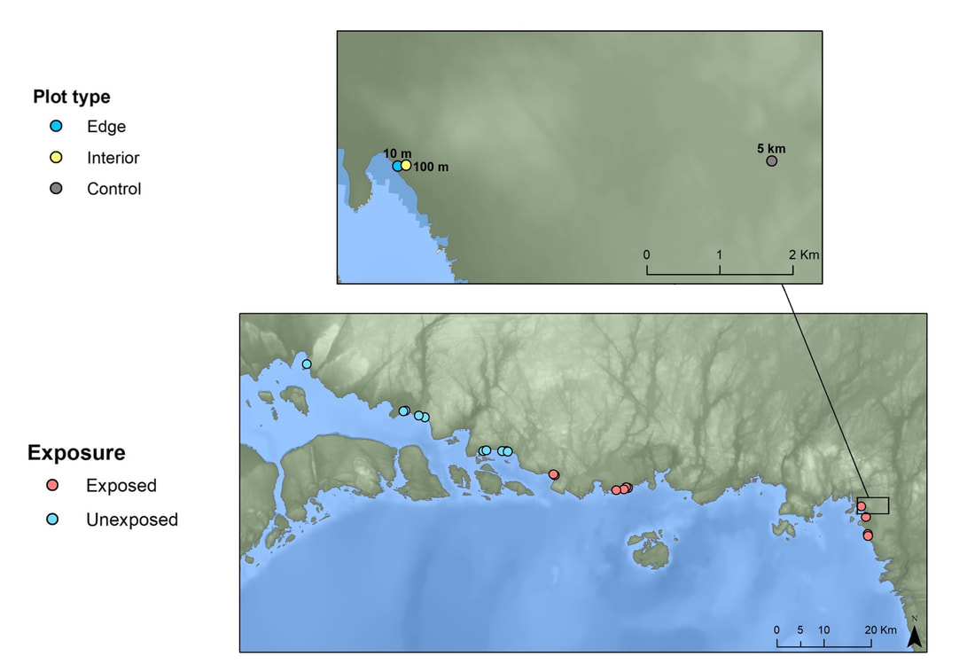
Figure 2. An inset map showing the distribution of 10 exposed and 10 unexposed sites (below) and how plot types were laid out from the shoreline (above; 10 m, 100 m, and 5 km inland).
Data Collection
We initially stratified sites by exposure class, where shorelines with no islands offshore were considered exposed to Lake Superior’s cooling effect while those with islands were unexposed. We then divided each site into 10 m (edge), 100 m (interior), and ≥5 km (control) plots perpendicular to the shoreline (Fig. 2). We used the 10 m plots to note the edge effects at the shore, 100 m plots to monitor the cooling effect inland, and control plots to represent forests likely unaffected by the lake’s cooling effect. We first chose these plots with Google Earth, but later surveyed them on the ground to determine that they were accessible and/or appropriate for our study. At each of the plot types, we measured 10 m^2 circular plots (Fig. 4) and recorded tree species within the plot and their respective Diameter at Breast Height (DBH) for those greater than 7 cm. In total, we sampled 10 sites at each of the exposed and unexposed site types, each of which included three different plots based on distance from shore. As such, we sampled 1,850 trees at a total of 60 plots from June to July, 2021.
Statistical Analysis
Because we had two or more treatment levels and a continuous dependent variable, we used Analysis of Variance (ANOVA) for our statistical analysis. This allowed us to see if any of our treatment levels (exposure or plot type, separately) were significantly different from each other. While our dependent variable data did not meet the assumptions of normality or homogeneity of variances, ANOVA is fairly robust against these assumptions owing to the central limit theorem. We log-transformed our abundance and DBH data in an attempt to adjust for the violations, but the transformations were of negligible difference on the output of our ANOVA.
